17  Bit-Plane Representations

Question. What does a lattice point look like in binary?

17.1 Learning Objectives

By the end of this chapter, you should be able to:

• represent signed lattice coordinates with fixed-width two’s-complement bits;
• extract bit planes from an integer vector;
• reconstruct signed integers from bit planes;
• identify the D4 least-significant-bit constraint;
• connect bit planes to Reed-Muller codewords;
• explain compression implications of constrained low bits.

17.2 Prerequisites

This chapter assumes D4 parity from Chapter 6 and Reed-Muller codewords from Chapter 16.

17.3 Running Example

Use the D4 point:

\[ u = (1,\;0,\;-2,\;3). \]

This is the running valid D4 vector from earlier chapters — an integer point that can be stored as bits.

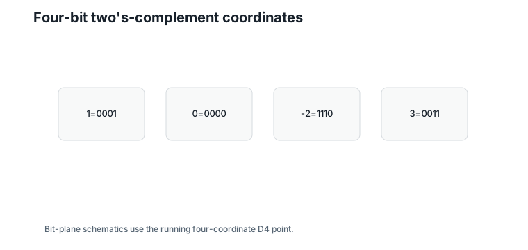
With four-bit two’s-complement encoding:

Value	Bits
1	0001
0	0000
-2	1110
3	0011

17.4 Binary Integers

Two’s-complement stores signed integers by wrapping negative values modulo \(2^B\), where \(B\) is the bit width.

For \(B = 4\):

\[ -2 \equiv 14 \pmod {16}. \]

The stored unsigned pattern for \(-2\) is 14, binary 1110: signed integers wrap around a finite ring, and fixed-width storage is reversible only inside its representable range.

Figure 17.1 shows the four-bit view.

Figure 17.1: Signed integers are represented by fixed-width bit patterns.

17.5 Bit Planes

A bit plane collects one bit position across all coordinates.

For \(u = (1,0,-2,3)\), the planes from least significant to most significant are:

Plane	Bits
0	\((1, 0, 0, 1)\)
1	\((0, 0, 1, 1)\)
2	\((0, 0, 1, 0)\)
3	\((0, 0, 1, 0)\)

Figure 17.2 shows the layout.

Figure 17.2: Bit planes collect the same bit position across coordinates.

17.6 D4 Low-Bit Constraint

The least-significant bit plane is:

\[ (1,\;0,\;0,\;1). \]

Interpretation:

• Verbal: these are the coordinate parities of the D4 point.
• Geometric: this is the binary signature modulo \(2\mathbb{Z}^4\).
• Engineering: the LSB plane must be an even-parity Reed-Muller codeword.

The sum is:

\[ 1 + 0 + 0 + 1 = 2. \]

Interpretation:

• Verbal: the LSB plane has even parity.
• Geometric: it is one of the allowed binary cosets.
• Engineering: this plane is constrained and therefore compressible.

One detail makes this robust: bit 0 of a two’s-complement pattern equals the value modulo 2 at any bit width, because the wrap offset \(2^B\) is even. So the LSB-plane constraint does not depend on how many bits store each coordinate — parity survives the representation.

Figure 17.3 shows the constraint.

Figure 17.3: The least-significant bit plane of a D4 point is an even-parity codeword.

17.7 Higher Bit Planes

Higher planes are not arbitrary, but the simple D4 membership rule constrains the low plane most directly. Recursive lattices such as Barnes-Wall impose additional code constraints across multiple planes.

Chapter 16’s Construction A makes the eight-dimensional case concrete. For the lattice \(2\mathbb{Z}^8 + RM(1,3)\) — a scaled E8 — the LSB plane of every point must be one of the 16 codewords of the extended Hamming code, out of \(2^8 = 256\) possible eight-bit patterns. Identifying the plane costs \(\log_2 16 = 4\) bits instead of 8. Where D4 saved one bit per plane, E8 saves four: stronger codes constrain low bits harder, and the constraint is exactly the packing quality.

Figure 17.4 shows the idea.

Figure 17.4: Recursive lattices impose code constraints across multiple bit planes.

This is why bit-plane representations are more than a storage trick: they reveal algebraic structure hidden inside integer coordinates.

17.8 Coefficient Bit Planes Are Hierarchical Nested Lattice Quantization (HNLQ) Digits

One more identification closes a loop opened in Chapter 10. There, the HNLQ encoder wrote the generator coefficients \(z\) of a lattice point in \(M\)-digit two’s complement, and each digit plane became an index \(b_m\). That is precisely this chapter’s construction — bit planes with the signed top plane — applied in coefficient space instead of coordinate space:

\[ \text{HNLQ digits} = \text{bit planes of } z, \qquad \text{coordinate planes} = \text{bit planes of } u = Gz. \]

These two sets of planes should not be confused. HNLQ digit planes live in generator-coefficient space; the Reed-Muller constraints discussed above live in coordinate space. The linear map \(G\) carries coefficient digit planes to digit representatives \(\tilde{c}_b = G\,\mathrm{bits}(b)\) before the weighted sum is formed. After those weighted representatives are added, carries can change the ordinary coordinate bit planes of \(u = Gz\).

So the hierarchy of Chapter 10, the quotients of Chapter 9, and the bit planes of this chapter are one structure seen from related but not identical angles: each HNLQ digit is a coset index, each coset index is a coefficient bit plane, and the coordinate bit planes carry the Reed-Muller constraints of Chapter 16. Keeping the two coordinate systems separate is what makes the unification useful rather than misleading.

17.9 Compression Implications

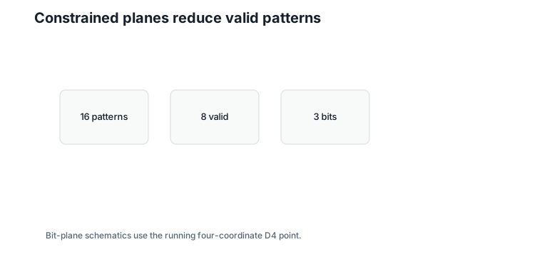
If bit planes were arbitrary, each plane would need to store all four bits independently. But the LSB plane of D4 has only 8 valid patterns, not 16.

That means:

\[ \log_2 8 = 3 \]

bits identify the LSB plane, instead of 4 bits.

Interpretation:

• Verbal: the parity constraint saves one bit for the low plane of a four-coordinate block.
• Geometric: half the binary signatures are invalid.
• Engineering: code constraints can reduce metadata or enable validation. This is the same bit Chapter 6 promised: D4 keeps half the integer points, so its blocks carry one less bit of low-plane information.

Figure 17.5 shows this count.

Figure 17.5: Code constraints reduce the number of valid bit-plane patterns.

17.10 Worked Example

Reconstruct u from its four planes.

The column bit patterns are:

Coordinate	Bits	Value
1	0001	1
2	0000	0
3	1110	-2
4	0011	3

Reading the bits vertically recovers each signed coordinate exactly.

17.11 Algorithms

17.11.1 Algorithm 17.1: Extract Bit Planes

Input: signed integer vector and bit width.

Output: bit planes from least significant to most significant.

function bit_planes(u, width):
    for bit from 0 to width - 1:
        plane[bit] = ((u >> bit) & 1) for each coordinate
    return planes

Complexity and implementation notes:

Property	Cost
Time	\(O(B \cdot d)\) for bit width \(B\)
Memory	\(O(B \cdot d)\)
Offline preprocessing	None
Online inference cost	Bit extraction
Parallelism	Coordinates and planes are independent
GPU suitability	Good with packed bit operations
SIMD suitability	Excellent
Possible optimization	Store planes already packed

17.11.2 Algorithm 17.2: Check D4 LSB Constraint

Input: bit planes of a four-coordinate vector.

Output: whether the LSB plane is an even-parity codeword.

function d4_lsb_valid(planes):
    return sum(planes[0]) is even

Complexity and implementation notes:

Property	Cost
Time	\(O(d)\)
Memory	\(O(1)\)
Offline preprocessing	None
Online inference cost	One parity reduction over the LSB plane
Parallelism	Blocks are independent
GPU suitability	Excellent
SIMD suitability	Excellent; a popcount on the packed plane suffices
Possible optimization	Validate many packed planes per instruction

The executable reference implementation is in code/python/chapter_17_bit_planes.py.

17.12 Engineering Insight

Bit planes expose constraints that ordinary integer arrays hide. For D4, the LSB plane is a Reed-Muller codeword. For richer lattices, multiple planes can carry nested code constraints.

This matters for compression and validation. A bitstream can store constrained planes more compactly, and a decoder can reject impossible patterns early.

17.13 Historical Note and Further Reading

Bit-plane representations are common in compression and hardware design. The lattice-specific point is that planes are not independent: code-lattice constructions impose algebraic constraints across them.

17.14 Exercises

17.14.1 Conceptual Exercises

1. Why does the LSB plane of a D4 point have even parity?
2. Why is sign handling necessary for bit-plane reconstruction?
3. How can constraints reduce storage?

17.14.2 Worked Numerical Exercises

1. Extract four-bit planes for \((1,0,-2,3)\).
2. Extract the LSB plane of \((2,-2,2,0)\).
3. Count valid even-parity low-bit patterns in length 4.

17.14.3 Programming Exercises

1. Run python code/python/chapter_17_bit_planes.py.
2. Add support for eight-bit two’s-complement values.
3. Pack each bit plane into one integer.

17.14.4 Research Questions

1. Can bit-plane constraints accelerate HNLQ decoding?
2. Which planes of E8 carry useful code constraints?
3. How should bit-plane data be laid out for GPU kernels?

17.15 Common Mistakes

• Losing sign information by using unsigned binary without a convention.
• Treating bit planes as independent.
• Forgetting that Python’s display of negative integers is not fixed-width.
• Checking D4 parity on the wrong plane.

17.16 Summary

A D4 lattice point has a constrained least-significant bit plane. For \((1,0,-2,3)\), the LSB plane is \((1,0,0,1)\), an even-parity Reed-Muller codeword. Bit planes expose binary structure that generator-matrix notation hides.

17.17 Preview of Next Chapter

The final chapter asks whether computation itself can use these structured binary representations directly, and clearly separates established facts from research directions.

Conway, John H., and N. J. A. Sloane. 1999. Sphere Packings, Lattices and Groups. 3rd ed. Vol. 290. Grundlehren Der Mathematischen Wissenschaften. Springer.

Deisenroth, Marc Peter, A. Aldo Faisal, and Cheng Soon Ong. 2020. Mathematics for Machine Learning. Cambridge University Press.

Forney, G. David. 1988. “Coset Codes. I. Introduction and Geometrical Classification.” IEEE Transactions on Information Theory 34 (5): 1123–51.

Gauss, Carl Friedrich. 1801. Disquisitiones Arithmeticae. Fleischer.

Gersho, Allen, and Robert M. Gray. 1992. Vector Quantization and Signal Compression. Kluwer Academic Publishers.

Jacob, Benoit, Skirmantas Kligys, Bo Chen, et al. 2018. “Quantization and Training of Neural Networks for Efficient Integer-Arithmetic-Only Inference.” Proceedings of the IEEE/CVF Conference on Computer Vision and Pattern Recognition, 2704–13.

Kaplan, Iris, and Or Ordentlich. 2025. High-Rate Nested-Lattice Quantized Matrix Multiplication with Small Lookup Tables. https://arxiv.org/abs/2505.13164.

Linde, Yoseph, Andres Buzo, and Robert M. Gray. 1980. “An Algorithm for Vector Quantizer Design.” IEEE Transactions on Communications 28 (1): 84–95.

Viazovska, Maryna S. 2017. “The Sphere Packing Problem in Dimension 8.” Annals of Mathematics 185 (3): 991–1015.