9  Quotient Groups and Finite Codebooks

Question. How can infinitely many lattice points become exactly 16 or 256 codewords?

9.1 Learning Objectives

By the end of this chapter, you should be able to:

• explain why scaling does not create a finite codebook;
• use cosets to group infinitely many lattice points into finitely many classes;
• construct \(D4/2D4\) and count its 16 classes;
• choose deterministic representatives for those classes;
• build the finite Hierarchical Nested Lattice Quantization (HNLQ) codebook \(A_q\);
• assign stable codebook indices for offline lookup.

9.2 Prerequisites

This chapter assumes modulo arithmetic from Chapter 2, finite codebooks from Chapter 4, the D4 lattice from Chapter 6, and lattice quantization from Chapter 8.

9.3 Running Example

The running lattice is still D4, the dimension is still \(d = 4\), and the quotient radix is:

\[ q = 2. \]

Interpretation:

• Verbal: we will group D4 points by differences that are multiples of 2.
• Geometric: the coarse lattice \(2D4\) is a wider copy of D4.
• Engineering: \(q = 2\) should produce \(2^4 = 16\) codewords for each four-dimensional block.

The goal is to construct the complete finite codebook:

\[ A_2 = D4 \cap 2V. \]

Interpretation:

• Verbal: keep the D4 points that lie inside the doubled origin Voronoi region.
• Geometric: choose one compact representative from each \(D4/2D4\) class.
• Engineering: these representatives become the finite codewords stored in an offline table.

By the end of the chapter, every codeword has a deterministic index from 0 to 15.

9.4 Why Chapter 8 Was Not Enough

Chapter 8 gave the scaled lattice quantizer:

\[ \text{reconstruction} = \frac{1}{\beta}Q_L(\beta v). \]

Scaling changes the effective step size and therefore the distortion — Chapter 8’s whole story.

But the scaled reconstruction set is still infinite:

\[ \left\{\frac{1}{\beta}y : y \in L\right\}. \]

The grid spacing changes, but the grid never ends: no finite number of bits can index this set directly.

To get fixed-rate coding, we must group infinitely many lattice points into finitely many classes.

9.5 Start With Integers

Modulo arithmetic already solved this problem for integers.

The integers are infinite:

\[ \mathbb{Z} = \{\ldots,-2,-1,0,1,2,\ldots\}. \]

Storing an arbitrary integer needs an unbounded number of bits unless we restrict or group it.

Modulo 4 groups all integers into four classes:

\[ \mathbb{Z}/4\mathbb{Z} = \{0,1,2,3\}. \]

The infinite number line folds into four repeating positions, and a remainder modulo 4 costs exactly 2 bits.

Figure 9.1 shows this fold.

Figure 9.1: Integers grouped into four modulo classes.

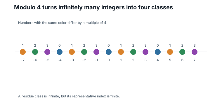
The class containing 1 is:

\[ 1 + 4\mathbb{Z} = \{\ldots,-7,-3,1,5,9,\ldots\}. \]

One stored index now represents infinitely many possible original integers — the pattern we need for lattices.

This is the pattern we need for lattices.

9.6 Vector Cosets

For integer vectors, the same idea applies coordinate by coordinate. In two dimensions, reducing modulo 2 gives:

\[ \mathbb{Z}^2 / 2\mathbb{Z}^2. \]

Two integer vectors are equivalent if they differ by an even vector; two parity bits index the four classes.

Figure 9.2 shows the four classes.

Figure 9.2: Two-dimensional integer vectors grouped by modulo-2 parity.

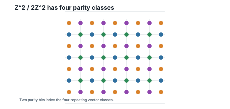
The four representatives can be:

\[ (0,0),\quad (0,1),\quad (1,0),\quad (1,1). \]

A finite table of four representatives replaces an infinite grid.

This is already a quotient codebook.

9.7 From Z4 to D4

D4 is not all of \(\mathbb{Z}^4\). It is the even-sum integer lattice:

\[ D4 = \{u \in \mathbb{Z}^4 : u_1 + u_2 + u_3 + u_4 \text{ is even}\}. \]

This is Chapter 6’s lattice; every codeword we build must satisfy the even-sum rule.

The coarse lattice \(2D4\) is:

\[ 2D4 = \{2u : u \in D4\}. \]

Doubling every D4 point creates a wider sublattice inside D4; differences in \(2D4\) will be treated as belonging to the same class.

Now we group D4 by \(2D4\). Two points are equivalent if their difference lies in \(2D4\):

\[ a \sim b \quad\text{when}\quad a - b \in 2D4. \]

Two points share a class when the coarse lattice can move one to the other; every class will need one stored representative and one index.

The quotient is written:

\[ D4 / 2D4. \]

Interpretation:

• Verbal: this is the set of equivalence classes of D4 points modulo \(2D4\).
• Geometric: it is one fundamental period of the D4 lattice under coarse-lattice shifts.
• Engineering: it is the finite codebook shape used by the \(q = 2\) HNLQ level.

9.8 Why There Are Sixteen Classes

Chapter 6 gave a generator matrix for D4. A D4 point can be written as:

\[ u = Gz. \]

The generator basis gives every lattice point integer coordinates, and coordinates give an easy indexing rule.

Modulo \(2D4\), only the parity of the four generator coefficients matters:

\[ z \bmod 2 \in \{0,1\}^4. \]

Interpretation:

• Verbal: each of the four generator coefficients has two possible residues.
• Geometric: the coarse lattice \(2D4\) forgets how many full pairs of generator steps were taken.
• Engineering: four bits give \(2^4 = 16\) possible quotient classes.

Therefore:

\[ |D4 / 2D4| = 16. \]

Interpretation:

• Verbal: the infinite lattice collapses into 16 classes.
• Geometric: one period of D4 under \(2D4\) contains 16 representatives.
• Engineering: one codebook index costs exactly 4 bits per four-dimensional block, or 1 bit per weight.

This is the first fixed-rate lattice codebook in the book.

9.9 Representatives

A quotient class is not a single vector. It is an infinite set of vectors. To build a codebook, we choose one representative from each class.

Representatives must be deterministic. If index 13 means one vector today and another vector tomorrow, a stored model becomes unreadable.

For Hierarchical Nested Lattice Quantization, the finite level codebook is:

\[ A_q = L \cap qV. \]

Interpretation:

• Verbal: keep lattice points inside the scaled origin Voronoi cell.
• Geometric: choose compact representatives around the origin.
• Engineering: this produces a small table that can be reused across blocks and hierarchy levels.

Read the display with care: taken literally, with the closed region, \(D4 \cap 2V\) contains more than 16 points, because boundary points shared between neighboring cells appear for several classes at once. The set becomes a 16-entry codebook only after a rule picks one point per class.

Boundary points therefore require a rule. In this book, a representative is chosen as follows: first consider all lattice points in the closed region \(qV\); within each quotient class, choose a minimum-norm point; if several points tie, choose the lexicographically largest vector.

The class with index 3 shows the rule earning its keep. That class contains all eight vectors of the form \((\pm 2, 0, 0, 0)\), \((0, \pm 2, 0, 0)\), \((0, 0, \pm 2, 0)\), \((0, 0, 0, \pm 2)\) — every one of them has norm 2, and every one of them sits exactly on the boundary of \(2V\), equidistant between the origin and a neighboring \(2D4\) point. Minimum norm alone cannot separate them; the lexicographic rule picks \((2, 0, 0, 0)\), and it will pick the same vector next year.

This is the same discipline Chapter 7 applied to nearest-point ties, now promoted from the encoder to the codebook itself: whenever geometry offers several equally valid answers, a deployed system must fix one by rule.

Figure 9.3 illustrates why the rule is needed.

Figure 9.3: Boundary tie-breaking assigns points on shared cell boundaries to one deterministic representative.

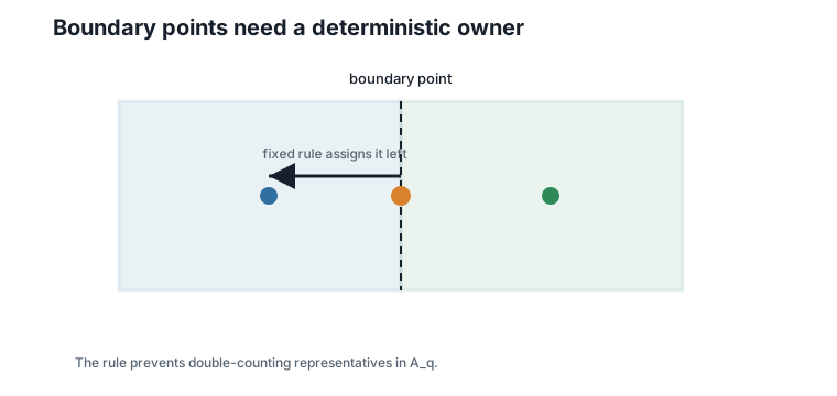
This rule is not decoration. Without it, a boundary point could be counted twice or not counted consistently.

9.10 The Complete D4, q = 2 Codebook

For the running example:

\[ A_2 = D4 \cap 2V. \]

Interpretation:

• Verbal: these are the D4 representatives in the doubled origin cell.
• Geometric: they form one compact period of D4 modulo \(2D4\).
• Engineering: this is the 16-entry finite codebook used by the \(q = 2\) level.

The stable index is the four-bit parity of the generator coefficients, read as a binary number.

Index \(b\)	Generator-coordinate bits	Representative \(c_b\)
0	0000	\((0, 0, 0, 0)\)
1	0001	\((0, 0, 1, 1)\)
2	0010	\((0, 0, 1, -1)\)
3	0011	\((2, 0, 0, 0)\)
4	0100	\((0, 1, -1, 0)\)
5	0101	\((0, 1, 0, 1)\)
6	0110	\((0, 1, 0, -1)\)
7	0111	\((0, 1, 1, 0)\)
8	1000	\((1, -1, 0, 0)\)
9	1001	\((1, 1, 1, -1)\)
10	1010	\((1, 1, 1, 1)\)
11	1011	\((1, 1, 0, 0)\)
12	1100	\((1, 0, -1, 0)\)
13	1101	\((1, 0, 0, 1)\)
14	1110	\((1, 0, 0, -1)\)
15	1111	\((1, 0, 1, 0)\)

Figure 9.4 summarizes the same table visually.

Figure 9.4: The sixteen representatives of the D4 modulo 2D4 codebook.

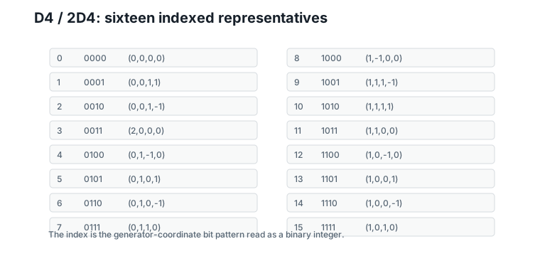
Every entry has even coordinate sum. Every pair of entries belongs to a different coset modulo \(2D4\). There are exactly 16 entries.

9.11 Reducing a Lattice Point to an Index

Suppose Chapter 7 decodes the first running block to:

\[ y_1 = (1,\;-2,\;2,\;-1). \]

This is the nearest D4 point for the first weight block — one point in the infinite lattice, not yet a finite index.

The generator coefficients for this point are:

\[ z = (1,\;-1,\;1,\;0). \]

These are the integer coordinates of \(y_1\) in the generator basis; their parities determine the quotient codebook index.

Modulo 2, the coefficient bits are:

\[ z \bmod 2 = (1,\;1,\;1,\;0). \]

Negative odd coefficients become residue 1, and the bit pattern 1110 is index 14.

So the finite representative is:

\[ c_{14} = (1,\;0,\;0,\;-1). \]

Interpretation:

• Verbal: \(c_{14}\) is the compact representative of the same quotient class.
• Geometric: the difference between \(y_1\) and \(c_{14}\) is a \(2D4\) shift.
• Engineering: storing index 14 is enough to identify the class.

Check the difference:

\[ y_1 - c_{14} = (0,\;-2,\;2,\;0) \in 2D4. \]

The decoded lattice point and its representative differ by a coarse-lattice point: the quotient index has discarded the coarse location, exactly as designed.

For the second decoded block:

\[ y_2 = (1,\;0,\;-2,\;3) \]

reduces to index 13 with representative:

\[ c_{13} = (1,\;0,\;0,\;1). \]

The two running blocks map to different quotient indices — this is how an infinite lattice point becomes a finite symbol.

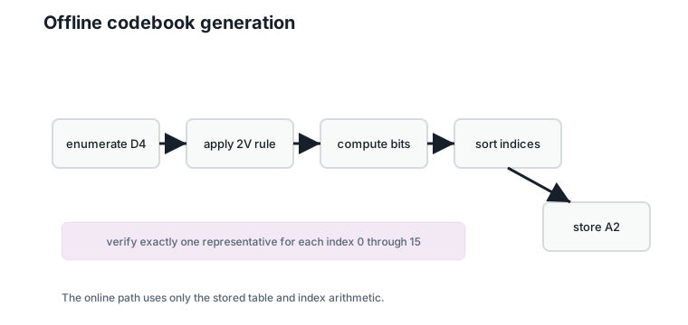
9.12 Offline Enumeration

The codebook is generated once and reused many times.

The offline procedure is:

1. Enumerate candidate D4 points in a small search window.
2. Keep only points in the closed region \(2V\).
3. Compute each point’s generator-coordinate parity bits.
4. Sort by the resulting index.
5. Verify that indices 0 through 15 appear exactly once.

Figure 9.5 shows the flow.

Figure 9.5: Offline codebook generation enumerates representatives, assigns indices, and stores a lookup table.

This table is now identical in form to a classical finite codebook: index in, representative out.

The difference is how the table was constructed. Classical vector quantization usually learns or chooses arbitrary codewords. Here, quotient structure guarantees the count and the indexing rule.

9.13 Nearest Representative Search

Once \(A_2\) is a finite codebook, we can also search it directly:

\[ b = \arg\min_j \|v - c_j\|_2. \]

This is ordinary finite-codebook nearest-neighbor search; for 16 entries, brute force is cheap.

This search and quotient reduction answer different questions:

• Nearest-lattice decoding followed by quotient reduction maps an arbitrary lattice point to its coset index.
• Brute-force search over \(A_2\) chooses the nearest compact codeword directly.

Both are useful. HNLQ will use finite codebooks inside a hierarchy, where residuals are kept near the origin. In that setting, compact representatives are exactly what we want.

9.14 Worked Example

Generate the codebook and encode the two Chapter 7 decoded lattice points.

The finite codebook has:

\[ |A_2| = 16. \]

Interpretation:

• Verbal: there are sixteen representatives.
• Geometric: one representative is chosen from each period of D4 under 2D4.
• Engineering: one block index costs 4 bits.

The first decoded lattice point reduces as:

Quantity	Value
Decoded lattice point	\((1, -2, 2, -1)\)
Generator coefficients	\((1, -1, 1, 0)\)
Bits	1110
Index	14
Representative	\((1, 0, 0, -1)\)
Difference	\((0, -2, 2, 0) \in 2D4\)

The second decoded lattice point reduces as:

Quantity	Value
Decoded lattice point	\((1, 0, -2, 3)\)
Generator coefficients	\((1, 1, -2, 1)\)
Bits	1101
Index	13
Representative	\((1, 0, 0, 1)\)
Difference	\((0, 0, -2, 2) \in 2D4\)

These two indices are not yet a full quantized model. They are one level of a quotient codebook. Chapter 10 will stack such levels hierarchically.

9.15 Algorithms

9.15.1 Algorithm 9.1: Generate A2 for D4

Input: the D4 membership test, the nearest-D4 decoder, and \(q = 2\).

Output: a 16-entry codebook indexed from 0 to 15.

function generate_A2_D4():
    entries = empty map
    for candidate in bounded integer search window:
        if candidate is not in D4:
            continue
        if candidate is not in the closed region 2V:
            continue
        bits = generator_coefficients(candidate) mod 2
        index = binary_integer(bits)
        keep candidate as one option for this index
    for each index:
        choose the minimum-norm candidate
        break ties by lexicographically largest vector
    require entries contain exactly indices 0 through 15
    return entries sorted by index

Complexity and implementation notes:

Property	Cost
Time	\(O(W^d)\) for an offline search window of width \(W\)
Memory	\(O(q^d)\) for the output codebook
Offline preprocessing	Required once per lattice/radix choice
Online inference cost	None for generation; lookup is \(O(1)\)
Parallelism	Candidate tests are independent
GPU suitability	Usually unnecessary for \(q = 2\), but enumeration is parallel
SIMD suitability	Good for batched membership and decoder checks
Possible optimization	Derive representatives algebraically instead of searching

9.15.2 Algorithm 9.2: Reduce a D4 Point Modulo 2D4

Input: a lattice point \(u\) in D4.

Output: a quotient index and representative.

function reduce_D4_mod_2D4(u):
    z = generator_coefficients(u)
    bits = z mod 2
    index = binary_integer(bits)
    representative = A2[index]
    return index, representative

Complexity and implementation notes:

Property	Cost
Time	\(O(d)\) for coefficient extraction and parity
Memory	\(O(1)\) beyond the codebook
Offline preprocessing	Requires the 16-entry \(A_2\) table
Online inference cost	A few integer operations and one table lookup
Parallelism	Excellent across blocks
GPU suitability	Excellent; table fits in constant or shared memory
SIMD suitability	Excellent for packed block indices
Possible optimization	Compute coefficient parity directly from coordinates

9.15.3 Algorithm 9.3: Nearest Representative Search

Input: target vector \(v\) and finite codebook \(A_2\).

Output: index of the nearest representative.

function nearest_representative(v, A2):
    best_index = 0
    best_distance = squared_distance(v, A2[0])
    for index from 1 to 15:
        current = squared_distance(v, A2[index])
        if current < best_distance:
            best_index = index
            best_distance = current
    return best_index

Complexity and implementation notes:

Property	Cost
Time	\(O(q^d d)\) for brute-force search over \(q^d\) representatives
Memory	\(O(q^d d)\) for the codebook
Offline preprocessing	Codebook generation
Online inference cost	16 distance computations for D4, \(q = 2\)
Parallelism	Distances are independent reductions
GPU suitability	Good for many blocks, but table lookup is often cheaper inside HNLQ
SIMD suitability	Good; all representatives are short vectors
Possible optimization	Use nearest-lattice decoding plus quotient reduction when the target is already decoded to D4

The executable reference implementation is in code/python/chapter_09_quotient_codebooks.py.

9.16 Engineering Insight

This chapter is the fixed-rate turning point.

Scaling adjusts distortion, but it does not determine how many symbols the encoder can emit. Quotients do. For D4 and \(q = 2\), the quotient \(D4/2D4\) has exactly 16 classes, so the codebook has exactly 16 representatives and the index costs exactly 4 bits per block.

The deterministic representative rule matters as much as the count. In a deployed model, index 14 must always decode to the same vector. Boundary tie-breaking, sorted indexing, and offline verification are therefore part of the mathematical construction, not implementation trivia.

This is why quotient codebooks are useful for inference: they give a small table, stable indices, predictable bit rate, and enough algebraic structure for the hierarchy in the next chapter.

9.17 Historical Note and Further Reading

Quotient and coset viewpoints are standard in lattice coding. Forney’s coset-code work is a classical entry point for the coding perspective, while Conway and Sloane provide the lattice background (Forney 1988; Conway and Sloane 1999). The contribution here is pedagogical and systems-oriented: we use quotients to explain how a lattice quantizer becomes a finite neural-network codebook.

9.18 Exercises

9.18.1 Conceptual Exercises

1. Why does \(D4/2D4\) have 16 classes instead of 8?
2. Why must a representative rule be deterministic?
3. What is the difference between a coset and a representative?

9.18.2 Worked Numerical Exercises

1. Compute the generator-coordinate parity bits for \((1, 0, -2, 3)\).
2. Verify that \((1, -2, 2, -1)\) and \((1, 0, 0, -1)\) are in the same coset modulo \(2D4\).
3. List the four classes of \(\mathbb{Z}^2 / 2\mathbb{Z}^2\).

9.18.3 Programming Exercises

1. Run python code/python/chapter_09_quotient_codebooks.py and print the complete 16-entry codebook.
2. Add a test that every representative has even coordinate sum.
3. Implement brute-force nearest search over the 16 representatives.

9.18.4 Research Questions

1. For larger \(q\), when does brute-force nearest-representative search become too expensive?
2. How should boundary tie-breaking be specified for a production quantizer?
3. What metadata is needed so a stored model can decode quotient indices years later?

9.19 Common Mistakes

• Confusing \(D4/2D4\) with the eight even-parity signatures of D4 modulo \(2\mathbb{Z}^4\).
• Treating representatives as arbitrary choices without stable indices.
• Forgetting that boundary points need a deterministic rule.
• Assuming the compact representative preserves the original coarse lattice location.
• Using nearest representative search and quotient reduction interchangeably without checking which problem is being solved.

9.20 Summary

Quotient groups turn an infinite lattice into a finite set of classes. For the running D4, \(q = 2\) example, \(D4/2D4\) has exactly 16 classes. The finite codebook \(A_2 = D4 \cap 2V\) chooses one deterministic representative from each class and assigns stable indices 0 through 15.

The running decoded lattice points reduce to indices 14 and 13. This is the first point in the book where lattice quantization has a fixed codebook size and a predictable number of bits.

9.21 Preview of Next Chapter

Next we stack these small quotient codebooks hierarchically. Hierarchical Nested Lattice Quantization will represent larger effective codebooks as combinations of small indexed representatives.

Conway, John H., and N. J. A. Sloane. 1999. Sphere Packings, Lattices and Groups. 3rd ed. Vol. 290. Grundlehren Der Mathematischen Wissenschaften. Springer.

Deisenroth, Marc Peter, A. Aldo Faisal, and Cheng Soon Ong. 2020. Mathematics for Machine Learning. Cambridge University Press.

Forney, G. David. 1988. “Coset Codes. I. Introduction and Geometrical Classification.” IEEE Transactions on Information Theory 34 (5): 1123–51.

Gauss, Carl Friedrich. 1801. Disquisitiones Arithmeticae. Fleischer.

Gersho, Allen, and Robert M. Gray. 1992. Vector Quantization and Signal Compression. Kluwer Academic Publishers.

Jacob, Benoit, Skirmantas Kligys, Bo Chen, et al. 2018. “Quantization and Training of Neural Networks for Efficient Integer-Arithmetic-Only Inference.” Proceedings of the IEEE/CVF Conference on Computer Vision and Pattern Recognition, 2704–13.

Kaplan, Iris, and Or Ordentlich. 2025. High-Rate Nested-Lattice Quantized Matrix Multiplication with Small Lookup Tables. https://arxiv.org/abs/2505.13164.

Linde, Yoseph, Andres Buzo, and Robert M. Gray. 1980. “An Algorithm for Vector Quantizer Design.” IEEE Transactions on Communications 28 (1): 84–95.

Viazovska, Maryna S. 2017. “The Sphere Packing Problem in Dimension 8.” Annals of Mathematics 185 (3): 991–1015.