14  Beyond D4: Higher-Dimensional Lattices

Question. Why stop at D4?

14.1 Learning Objectives

By the end of this chapter, you should be able to:

• generalize the D4 parity lattice to D_n;
• describe E8 as two shifted D8 shells;
• implement a simple nearest-E8 decoder;
• compare \(D4 \times D4\) and E8 on the running 8-weight vector;
• explain coding gain and packing density qualitatively;
• reason about the tradeoff between geometry and decoder complexity.

14.2 Prerequisites

This chapter assumes D4 membership from Chapter 6, nearest-D_n decoding from Chapter 7, and the eight-weight running example.

14.3 Running Example

Until now, the eight weights were two separate D4 blocks:

\[ w = (0.73,\;-1.84,\;2.11,\;-0.45,\;1.27,\;0.08,\;-2.36,\;3.14). \]

Interpretation:

• Verbal: the same eight values can be treated as two blocks or one larger block.
• Geometric: \(D4 \times D4\) uses two independent four-dimensional cells; E8 uses one eight-dimensional cell.
• Engineering: a larger block may reduce distortion, but the decoder and lookup tables become more complex.

14.4 Review of D4 and Dn

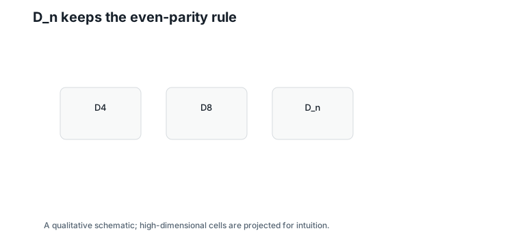
The D_n lattice is:

\[ D_n = \{u \in \mathbb{Z}^n : u_1 + \cdots + u_n \text{ is even}\}. \]

Interpretation:

• Verbal: D_n is the even-sum integer lattice in dimension \(n\).
• Geometric: it keeps one parity layer of the integer grid.
• Engineering: the Chapter 7 round-and-fix decoder works for any \(n\).

For \(n = 4\), this is D4. For \(n = 8\), it is D8.

Figure 14.1 shows the family idea.

Figure 14.1: The Dn family generalizes D4 by keeping the same even-parity rule in higher dimension.

14.5 Constructing E8

One useful construction of E8 is:

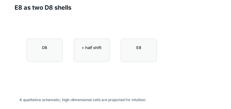
\[ E8 = D8 \cup \left(D8 + \left(\frac12,\ldots,\frac12\right)\right). \]

Interpretation:

• Verbal: E8 is the union of the D8 lattice and a half-shifted copy of D8.
• Geometric: the half-shift fills holes in the D8 packing.
• Engineering: nearest-E8 decoding can try two nearest-D8 decodes and choose the closer candidate.

Figure 14.2 illustrates the two-shell view.

Figure 14.2: E8 can be viewed as D8 plus a half-shifted copy of D8.

This construction is enough for an implementation overview. It is not the only way to define E8.

14.6 Nearest E8 Decoder

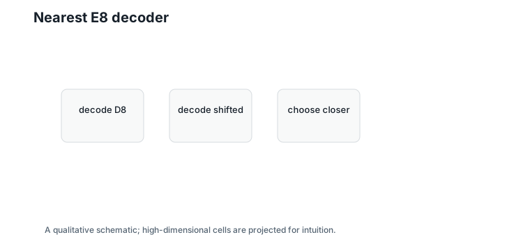
Given a target \(v\), compute two candidates:

\[ y_0 = Q_{D8}(v), \]

Interpretation:

• Verbal: decode directly to the nearest D8 point.
• Geometric: this checks the integer even-parity shell.
• Engineering: this is one call to the D_n decoder.

and:

\[ y_1 = \left(\frac12,\ldots,\frac12\right) + Q_{D8}\left(v - \left(\frac12,\ldots,\frac12\right)\right). \]

Interpretation:

• Verbal: shift the target down by half, decode to D8, then shift back.
• Geometric: this checks the half-shifted shell.
• Engineering: this is a second call to the same decoder.

Choose the closer candidate.

Figure 14.3 shows the two-candidate flow.

Figure 14.3: Nearest E8 decoding compares the D8 candidate with the half-shifted D8 candidate.

14.7 Running Comparison

The product-lattice result from two independent D4 decodes is:

\[ (1,\;-2,\;2,\;-1,\;1,\;0,\;-2,\;3). \]

Interpretation:

• Verbal: this is the Chapter 7 result applied to both blocks.
• Geometric: the vector lies in \(D4 \times D4\).
• Engineering: it uses two small four-dimensional decoders.

Its squared error is:

\[ 0.6416. \]

Interpretation:

• Verbal: this is the total squared error across all eight coordinates.
• Geometric: it is the squared distance from \(w\) to the product-lattice reconstruction.
• Engineering: it is the baseline for the E8 comparison.

The two E8 candidates are:

Candidate	Point	Squared error
D8 shell	\((1, -2, 2, -1, 1, 0, -2, 3)\)	0.6416
half-shifted shell	\((0.5, -1.5, 2.5, -0.5, 1.5, 0.5, -2.5, 3.5)\)	0.7016

For this particular vector, E8 chooses the same point as \(D4 \times D4\).

Figure 14.4 summarizes the result.

Figure 14.4: The running vector gets the same nearest point from D4 x D4 and E8 in this example.

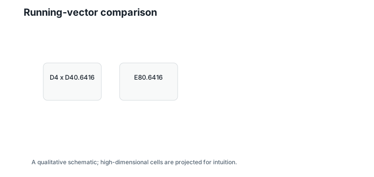
This is not a failure of E8. Better geometry improves average behavior, not every individual target.

14.8 Coding Gain and Packing Density

Before the numbers, note the containment ladder hiding in this chapter. A vector whose two block sums are both even has an even total sum, so \(D4 \times D4\) is a sublattice of D8 — the eight-dimensional parity lattice is already richer than two independent four-dimensional ones, because it also admits blocks whose sums are both odd. And E8 contains D8 by construction, adding the half-shifted shell that fills D8’s deepest holes. Each step of \(D4 \times D4 \subset D8 \subset E8\) adds points without changing the even-parity spirit.

Packing density asks how much space is covered by equal-radius spheres around lattice points before spheres overlap. Quantization gain asks how small the average squared error is over a cell.

Dense lattices are attractive because their cells are more sphere-like. More sphere-like cells usually reduce average quantization error.

For E8 the numbers are remarkable, and they extend Chapter 6’s fair-comparison discipline. The E8 generator has determinant 1 — exactly one lattice point per unit volume, the same density as the cubic grid \(\mathbb{Z}^8\). Yet its nearest points are \(\sqrt{2} \approx 1.41\) apart instead of 1, with 240 nearest neighbors. A 41% separation bonus at identical density is what eight-dimensional room to maneuver buys. This is not merely the best known construction: Viazovska proved that no sphere packing in eight dimensions — lattice or not — beats E8 (Viazovska 2017).

Figure 14.5 compares the idea qualitatively.

Figure 14.5: Better lattices have cells that are more sphere-like, improving average quantization behavior.

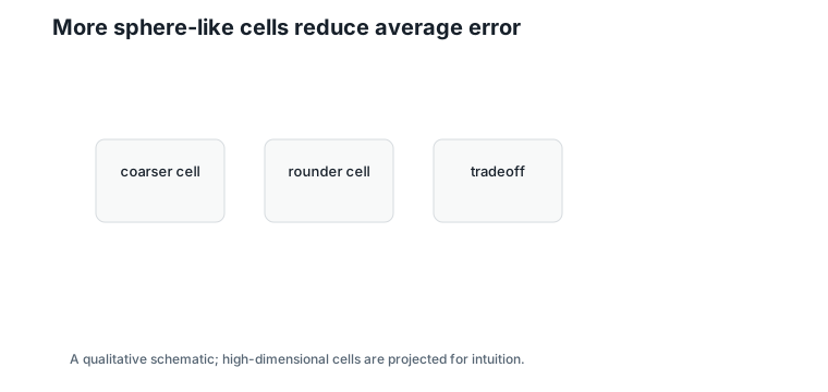
The practical question is whether the reduction in distortion is worth the cost of a larger block and a more complex decoder.

14.9 Practical Implications

D4 is small and SIMD-friendly. E8 has better geometry, but it doubles the block size and changes the lookup-table story.

Lattice	Block size	Decoder idea	Practical tradeoff
D4	4	round-and-fix	small, simple, easy LUTs
D_n	\(n\)	round-and-fix	scalable parity family
E8	8	two D8 decodes	better geometry, larger blocks
Leech	24	specialized	excellent geometry, much more complex

The Leech lattice is important historically and geometrically, but it is not a natural first implementation target for neural-network inference.

14.10 Worked Example

Run the E8 decoder on the running vector.

First shell:

\[ Q_{D8}(w) = (1,\;-2,\;2,\;-1,\;1,\;0,\;-2,\;3). \]

Interpretation:

• Verbal: direct D8 decoding gives an integer even-sum vector.
• Geometric: this lies on the unshifted shell.
• Engineering: this candidate costs one D_n decode.

Second shell:

\[ \left(\frac12,\ldots,\frac12\right) + Q_{D8}\left(w-\left(\frac12,\ldots,\frac12\right)\right) = (0.5,\;-1.5,\;2.5,\;-0.5,\;1.5,\;0.5,\;-2.5,\;3.5). \]

Interpretation:

• Verbal: the half-shifted shell gives a different candidate.
• Geometric: every coordinate is half-integer.
• Engineering: this candidate costs another D_n decode and a distance comparison.

The first candidate is closer, so nearest E8 returns the same reconstruction as D4 x D4 for this vector.

14.11 Algorithms

14.11.1 Algorithm 14.1: Nearest E8 Overview

Input: an eight-dimensional target vector \(v\).

Output: nearest point in E8.

function nearest_E8(v):
    h = (1/2, ..., 1/2)
    y0 = nearest_Dn(v)
    y1 = h + nearest_Dn(v - h)
    if distance(v, y0) <= distance(v, y1):
        return y0
    return y1

Complexity and implementation notes:

Property	Cost
Time	Two \(O(n)\) D_n decodes plus distance comparison
Memory	\(O(n)\) for candidates
Offline preprocessing	None
Online inference cost	Higher than D4, still structured
Parallelism	Two candidates and coordinate operations are parallelizable
GPU suitability	Good for batched blocks, but block size doubles
SIMD suitability	Good for 8-wide vectors
Possible optimization	Fuse candidate generation and distance computation

The executable reference implementation is in code/python/chapter_14_higher_lattices.py.

14.12 Engineering Insight

Better lattices can reduce distortion, but they also change the systems problem. E8 can be decoded efficiently, but an E8 Hierarchical Nested Lattice Quantization (HNLQ) table is an eight-dimensional object. Larger blocks may improve geometry while making lookup tables, cache placement, and calibration harder.

The right question is not “Which lattice is mathematically best?” The right question is “Which lattice gives the best accuracy-speed-memory tradeoff for a target inference system?”

14.13 Historical Note and Further Reading

The E8 and Leech lattices are central examples in the geometry of numbers and sphere packing. Conway and Sloane remain the standard reference for their structure and coding connections (Conway and Sloane 1999). This chapter uses only the minimal E8 construction needed to connect better geometry to quantization tradeoffs.

14.14 Exercises

14.14.1 Conceptual Exercises

1. Why does E8 contain a half-shifted copy of D8?
2. Why can a better lattice fail to improve one specific vector?
3. What changes in LUT design when block size grows from 4 to 8?

14.14.2 Worked Numerical Exercises

1. Verify the squared error 0.7016 for the half-shifted candidate.
2. Decode \((0.2, 0.2, \ldots, 0.2)\) with the two-candidate E8 rule.
3. Compare D8 and half-shifted candidates for a vector near \((0.5, \ldots, 0.5)\).

14.14.3 Programming Exercises

1. Run python code/python/chapter_14_higher_lattices.py.
2. Generate random vectors and count how often the half-shifted shell wins.
3. Time \(D4 \times D4\) decoding versus E8 decoding for many blocks.

14.14.4 Research Questions

1. When is the distortion gain of E8 worth the larger table structure?
2. How should E8 quotient representatives be indexed?
3. Are there hardware layouts that make 8-dimensional blocks natural?

14.15 Common Mistakes

• Assuming denser always means faster.
• Comparing D4 and E8 without fixing dimension and bit rate.
• Treating the Leech lattice as a practical default because it is geometrically famous.
• Forgetting that average gain does not guarantee every vector improves.

14.16 Summary

D4 belongs to the D_n family, and E8 can be built from D8 plus a half-shifted copy. A simple nearest-E8 decoder checks both shells and chooses the closer candidate.

For the running vector, E8 chooses the same point as \(D4 \times D4\), with squared error 0.6416. The lesson is the tradeoff: better lattice geometry can help average quantization, but larger blocks and more complex tables affect implementation.

14.17 Preview of Next Chapter

Next we look at Barnes-Wall lattices, where recursive structure offers another way to represent lattices beyond generator matrices.

Conway, John H., and N. J. A. Sloane. 1999. Sphere Packings, Lattices and Groups. 3rd ed. Vol. 290. Grundlehren Der Mathematischen Wissenschaften. Springer.

Deisenroth, Marc Peter, A. Aldo Faisal, and Cheng Soon Ong. 2020. Mathematics for Machine Learning. Cambridge University Press.

Forney, G. David. 1988. “Coset Codes. I. Introduction and Geometrical Classification.” IEEE Transactions on Information Theory 34 (5): 1123–51.

Gauss, Carl Friedrich. 1801. Disquisitiones Arithmeticae. Fleischer.

Gersho, Allen, and Robert M. Gray. 1992. Vector Quantization and Signal Compression. Kluwer Academic Publishers.

Jacob, Benoit, Skirmantas Kligys, Bo Chen, et al. 2018. “Quantization and Training of Neural Networks for Efficient Integer-Arithmetic-Only Inference.” Proceedings of the IEEE/CVF Conference on Computer Vision and Pattern Recognition, 2704–13.

Kaplan, Iris, and Or Ordentlich. 2025. High-Rate Nested-Lattice Quantized Matrix Multiplication with Small Lookup Tables. https://arxiv.org/abs/2505.13164.

Linde, Yoseph, Andres Buzo, and Robert M. Gray. 1980. “An Algorithm for Vector Quantizer Design.” IEEE Transactions on Communications 28 (1): 84–95.

Viazovska, Maryna S. 2017. “The Sphere Packing Problem in Dimension 8.” Annals of Mathematics 185 (3): 991–1015.